
How Multi-Column Statistics Work
The short answer: in the real world, only the first column works. When SQL Server needs data about the second column, it builds its own stats on that column instead (assuming they don’t already exist), and uses those two statistics together – but they’re not really correlated.
For the longer answer, let’s take a large version of the Stack Overflow database, create a two-column index on the Users table, and then view the resulting statistics:
|
1 2 3 4 5 6 7 |
DropIndexes; GO CREATE INDEX Location_Reputation ON dbo.Users(Location, Reputation); GO DBCC SHOW_STATISTICS('dbo.Users', 'Location_Reputation'); GO |
The output of DBCC SHOW_STATISTICS shows that we’ve got about 22 million rows in this table. So, what does the statistics histogram say about the relationships between locations and reputations?
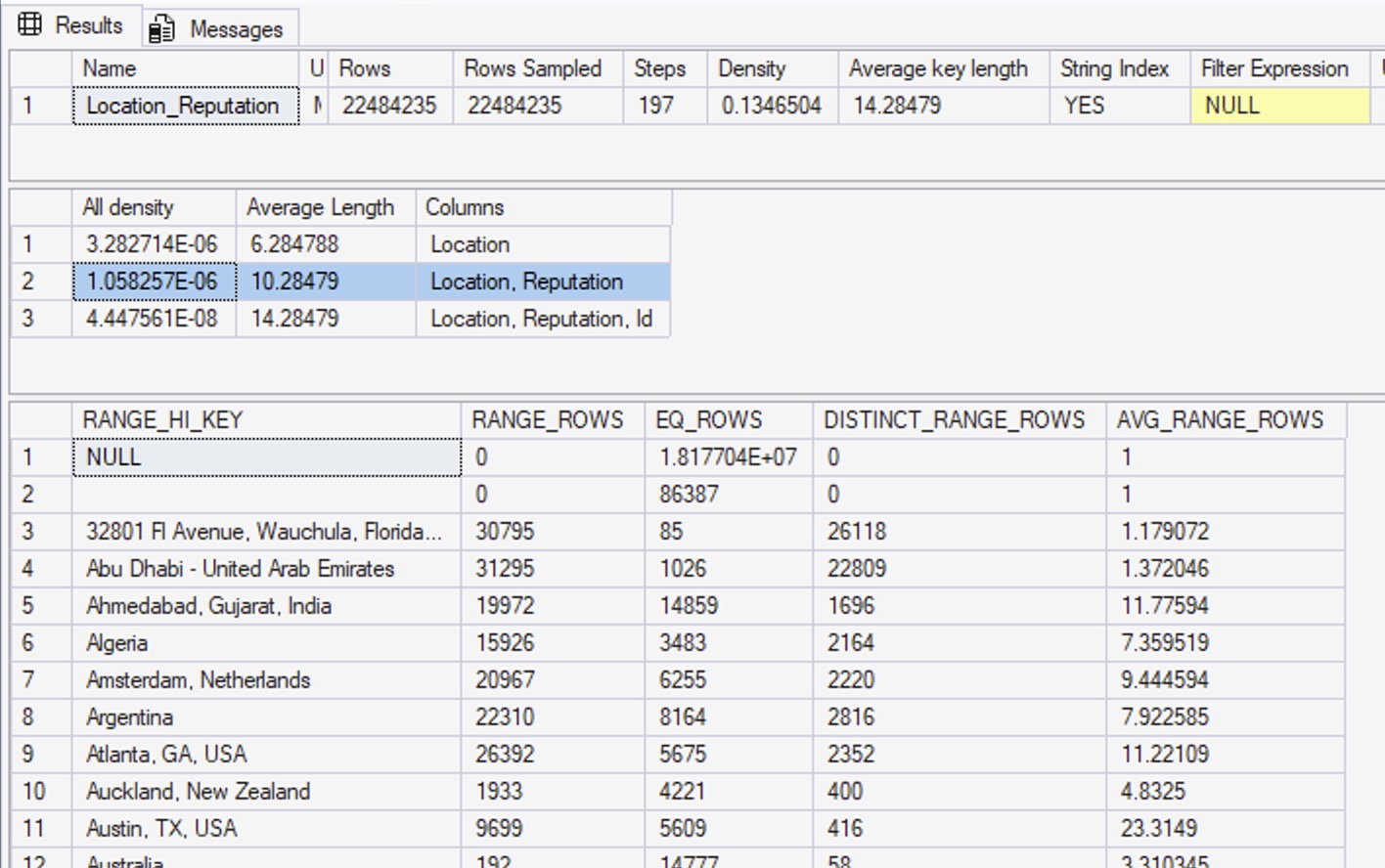
In the first result set, you can see that Rows = 22,484,235, and Rows Sampled = 22,484,235 – the same number. That means our statistics had a full scan, which is as good as they can possibly get.
The density vectors aren’t very useful.
The second result set are the density vectors – aka, the averages – and it has 3 rows. The first one says Location: all density = 3.282714E-06. If you take that number, times 22,484,235, you get 73.8093. That’s the density vector: if SQL Server needs to estimate how many rows are going to match for a given location, and it doesn’t know what the location is, it’ll estimate 73.8093.
Here’s an example query to prove that. I’m using a local variable to prevent SQL Server from sniffing the value, so it’ll have no idea what the @LocationUnknown value will be at compilation time:
|
1 2 3 4 5 |
DECLARE @LocationUnknown NVARCHAR(200) = N'Las Vegas, NV'; SELECT COUNT(*) FROM dbo.Users WHERE Location = @LocationUnknown; |
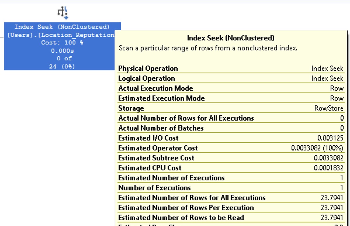
In the resulting query plan:
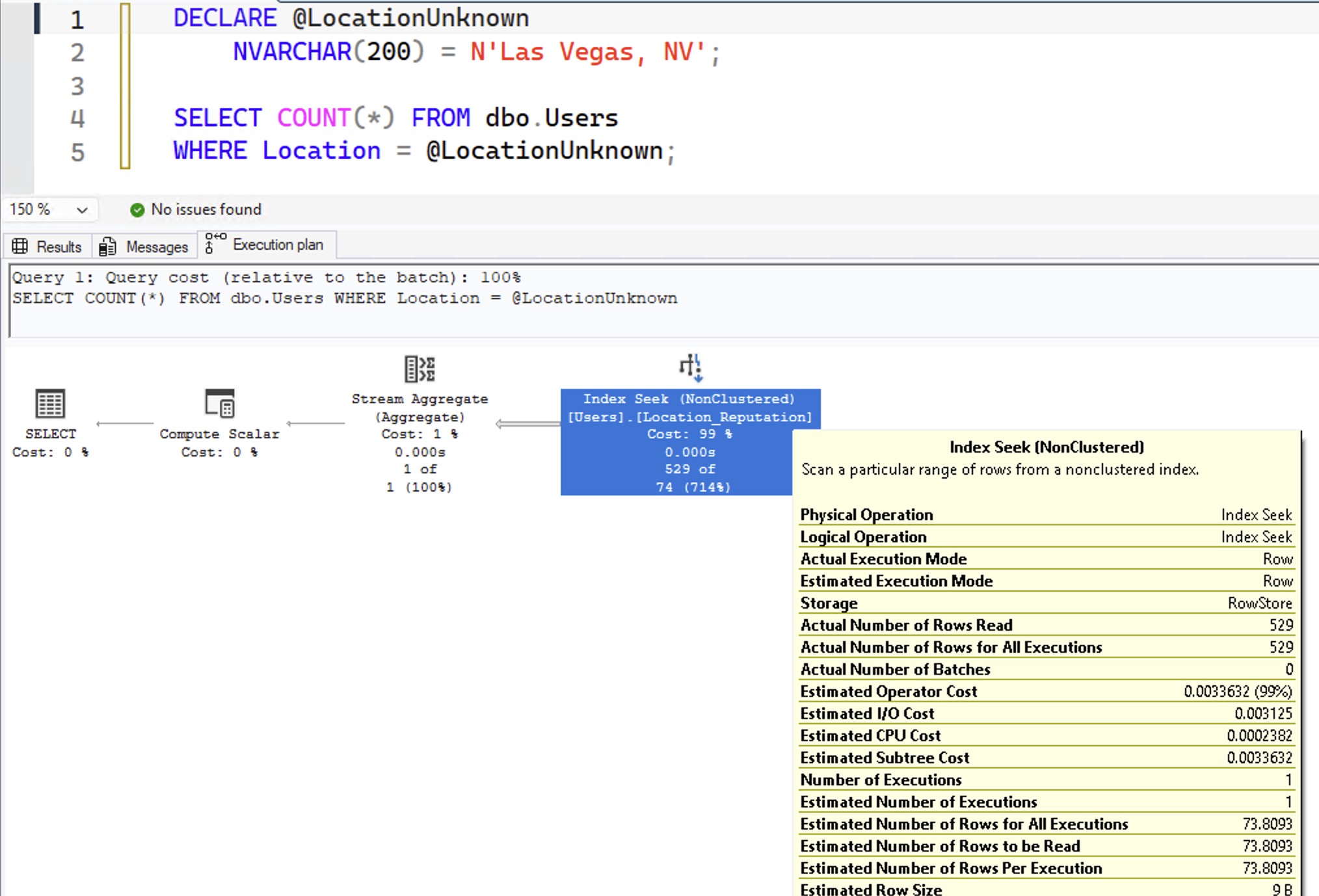
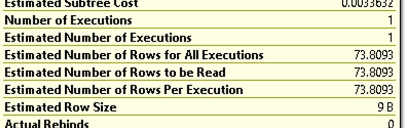
When you hover your mouse over the index seek and look at “Estimated Number of Rows Per Execution”, you get 73.8093:
Back to our DBCC SHOW_STATISTICS output. We explained that the first row was the density vector for Location alone – so what’s the second row, which says Location, Reputation?
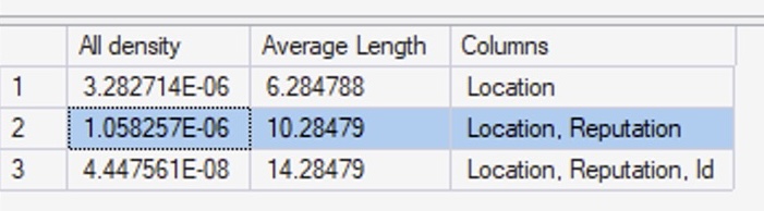
What’s that “1.058257E-06” number mean in the Location, Reputation column? Multiply that by the number of rows in the table (22,484,235) and you get 23.794. I bet you can see where I’m going with this:
|
1 2 3 4 5 6 |
DECLARE @LocationUnknown NVARCHAR(200) = N'Las Vegas, NV', @ReputationUnknown INT = 1234; SELECT COUNT(*) FROM dbo.Users WHERE Location = @LocationUnknown AND Reputation = @ReputationUnknown; |
Here’s our query plan, and bingo, 23.794 estimated rows:
If you’re searching for an unknown (or unpredictable before runtime) location and reputation combo, SQL Server uses the density vector in the histogram to calculate how many rows are going to match. SQL Server thinks that for any given location and reputation, no matter what values you pass in, they’re going to produce 23.7941.
At first, that sounds ridiculous: Reputation is an integer number. If you’re asking for equality searches on that number, and you’re passing in random numbers, there’s practically no way that estimate could be right. On “average”, maybe across thousands or millions of searches, this could be vaguely the average number – but it’s never going to be correct. It’s going to be wildly overestimated some times, and wildly underestimated at other times.
But what about the histogram?
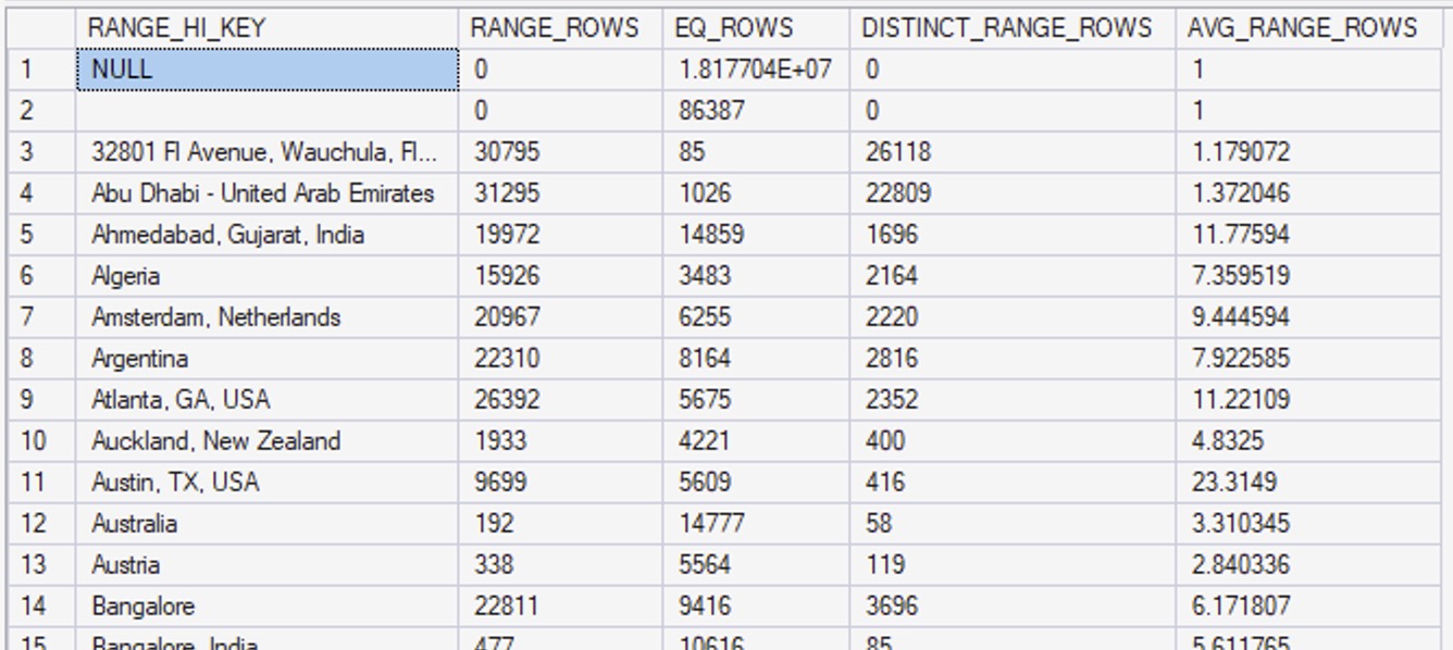
The next result set in DBCC SHOW_STATISTICS is the histogram, which contains the detailed list of up to 201 location values – because Location is the first column in our statistic:
Let’s scroll down to the Vegas area:
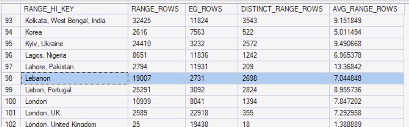
Las Vegas isn’t big enough of an outlier to get its own bucket, so if we query for the people who live in Las Vegas:
|
1 2 |
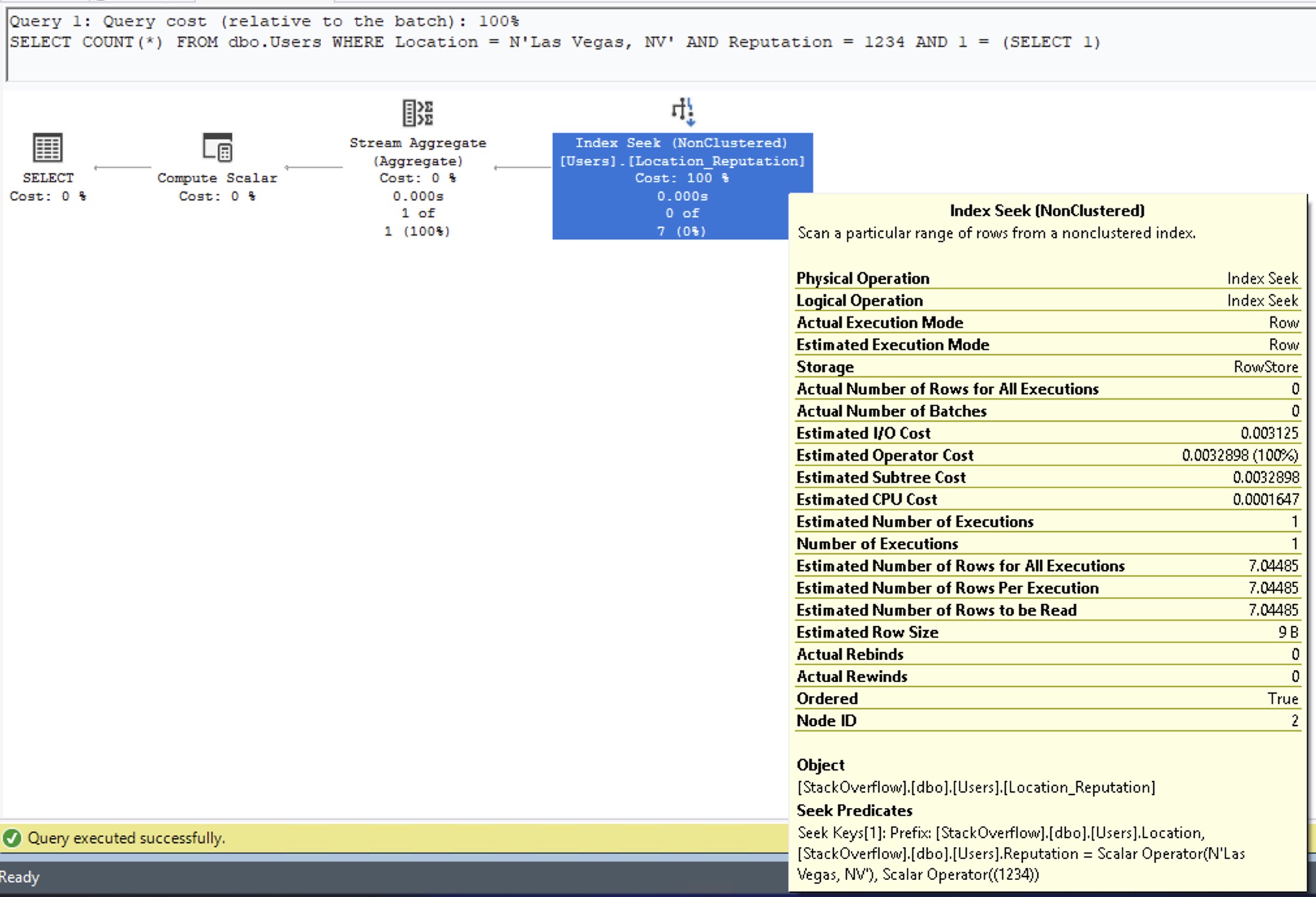
SELECT COUNT(*) FROM dbo.Users WHERE Location = N'Las Vegas, NV' AND 1 = (SELECT 1); |
Note that I’m using 1 = (SELECT 1) in order to prevent autoparameterization, which is a totally different subject for another day. Hover our mouse over the execution plan to see the estimated number of rows:
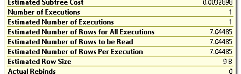
The 7.04485 estimate comes from our statistics. Scroll back up a couple of images, and note that in our statistics, I highlighted the row for Lebanon. “Las Vegas, NV” is somewhere between “Lahore, Pakistan” and “Lebanon” (it certainly feels that way on the highway sometimes), so SQL Server uses the AVG_RANGE_ROWS number of 7.044848.
When SQL Server is searching for an unknown Location, it uses the density vector. When it’s searching for a known location in between two range high keys, it uses the AVG_RANGE_ROWS number. So far, so good.
But what happens if we pass in a search for a known location AND a known reputation?
|
1 2 3 4 |
SELECT COUNT(*) FROM dbo.Users WHERE Location = N'Las Vegas, NV' AND Reputation = 1234 AND 1 = (SELECT 1); |
Before we look at the execution plan of that query, take a moment to review the statistics at play here. Which column is SQL Server going to use for its estimate?
Which column in the above screenshot tells SQL Server that any particular location has a higher or lower average reputation score, or how distributed the values are?
That’s right: there isn’t one!
This statistics histogram isn’t really about the second column of the object at all. It’s about the first column! Multi-column stats aren’t, really: they’re really just single-column stats!
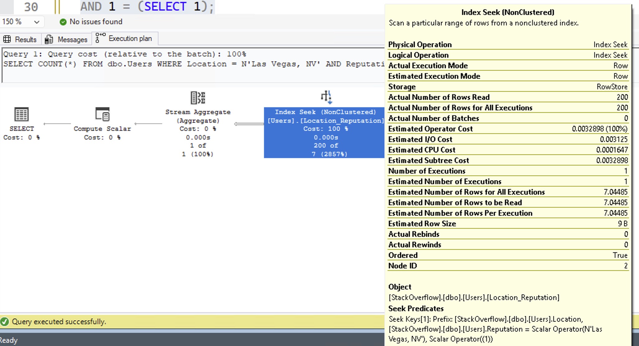
Here’s the part that’s kinda mind-blowing. Here’s the query plan for Las Vegas and 1234:
Look familiar? That’s a 7.04485 estimate. Exactly the same as if we weren’t filtering on reputation at all. It’s using the avg_range_rows from our statistics, giving us the exact same estimate that we got from just filtering on Location = Las Vegas.
The histogram values for the first column in our object is really useful. Subsequent columns, not so much.
The Reputation value I’m searching for doesn’t really matter here either. Let’s try one of the biggest values, Reputation = 1. You’ll see why this is important later:
The estimate is still 7.04485: exactly the same as not filtering by reputation at all. That’s… not great.
Things change a little for really big outliers.
Let’s try searching for the very biggest location value: India. If we search for just the location value (not a reputation yet), the histogram is useful because India’s one of our outliers:
|
1 2 3 |
SELECT COUNT(*) FROM dbo.Users WHERE Location = N'India' AND 1 = (SELECT 1); |
The resulting execution plan estimates are absolutely bang on:
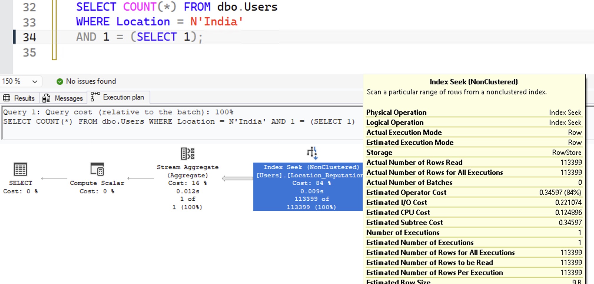
Then add in a filter for a given reputation number, and here I’m going to do both 1234 and 1 back to back:
|
1 2 3 4 5 6 7 8 9 |
SELECT COUNT(*) FROM dbo.Users WHERE Location = N'India' AND Reputation = 1234 AND 1 = (SELECT 1); SELECT COUNT(*) FROM dbo.Users WHERE Location = N'India' AND Reputation = 1 AND 1 = (SELECT 1); |
And whaddya know: now our estimates are not 7.04485, unlike Las Vegas:
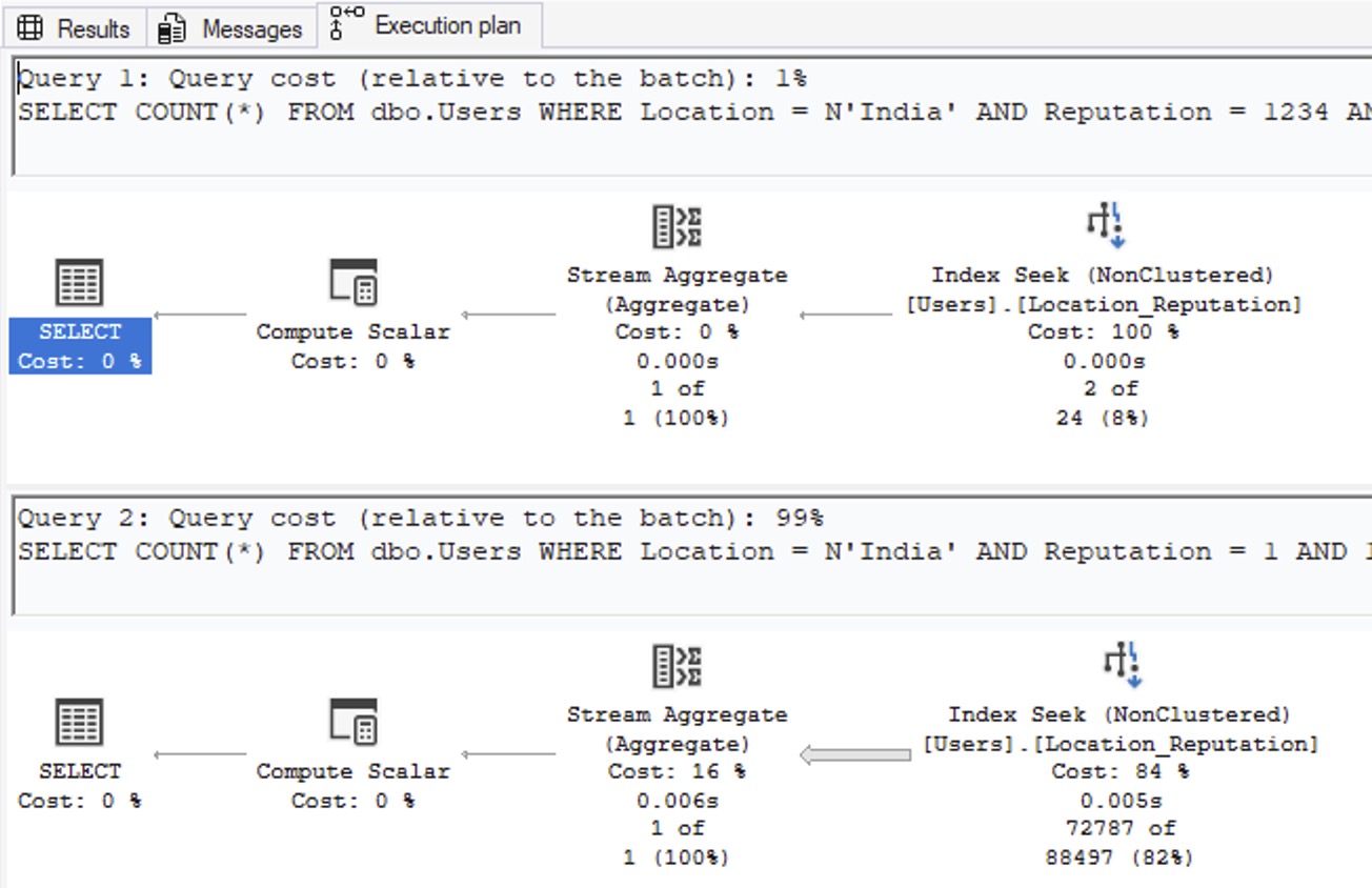
SQL Server manages to figure out that India is not only huge, but also that Reputation = 1 is huge. So, how’d it do that? Right-click on the SELECT operator of the second query, go into Properties, and then OptimizerStatsUsage:
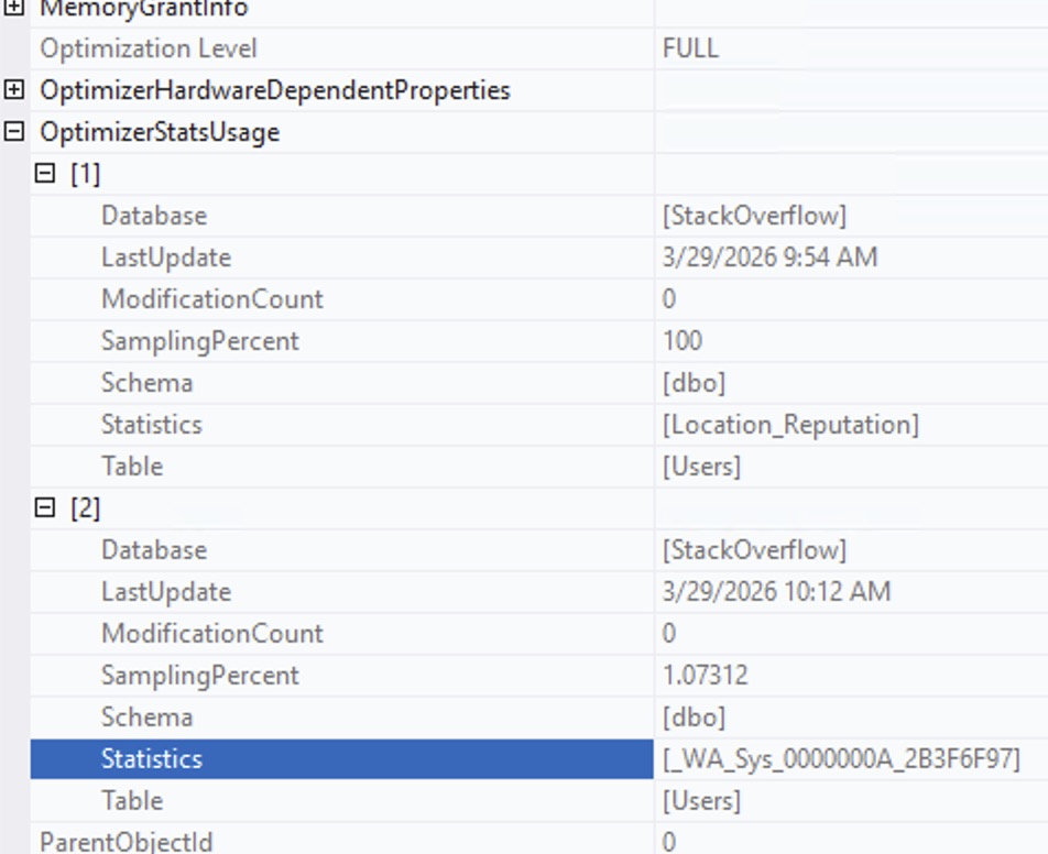
SQL Server didn’t just use the stat on Location_Reputation. In order to understand that Reputation = 1 is an outlier, it also automatically created a statistic on the Reputation column separately because the Reputation data in the Location_Reputation statistic just wasn’t useful enough.
Multi-column stats just don’t help much by themselves.
To really prove it, let’s set up an artificial scenario. Let’s say that everyone in China has really high reputation. And, just to give SQL Server the best defenses possible, let’s create a multi-column index (and therefore stat) on Reputation, Location. Hell, let’s even update statistics on Users so that our existing Location, Reputation stat completely understands that China’s where the smart people are at:
|
1 2 3 4 5 6 7 |
UPDATE dbo.Users SET Reputation = 1000000 WHERE Location = N'China'; CREATE INDEX Reputation_Location ON dbo.Users(Reputation, Location); UPDATE STATISTICS dbo.Users WITH FULLSCAN; |
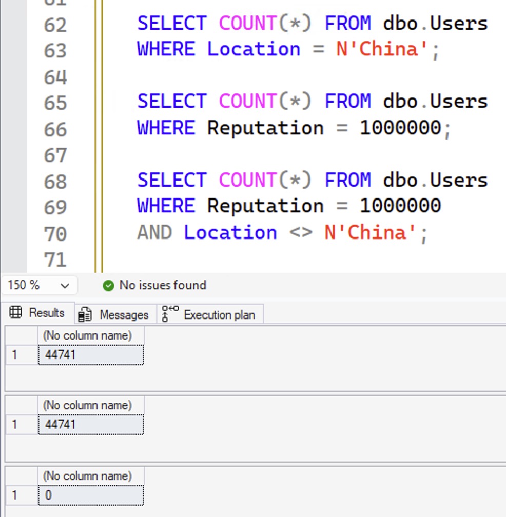
If that was a Venn diagram, we would now have a perfect circle: all of the people in China have exactly 1,000,000 reputation points, and the only people with exactly 1,000,000 reputation points are in China:
|
1 2 3 4 5 6 7 8 9 |
SELECT COUNT(*) FROM dbo.Users WHERE Location = N'China'; SELECT COUNT(*) FROM dbo.Users WHERE Reputation = 1000000; SELECT COUNT(*) FROM dbo.Users WHERE Reputation = 1000000 AND Location <> N'China'; |
The results:
So now, let’s ask SQL Server:
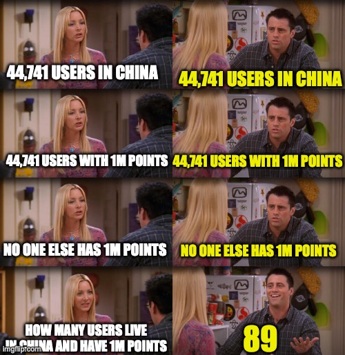
- How many people do you THINK live in China?
- How many people do you THINK have 1,000,000 reputation points?
- How many people do you THINK live in China, AND have 1,000,000 points?
|
1 2 3 4 5 6 7 8 9 |
SELECT COUNT(*) FROM dbo.Users WHERE Location = N'China' AND 1 = (SELECT 1); SELECT COUNT(*) FROM dbo.Users WHERE Reputation = 1000000 AND 1 = (SELECT 1); SELECT COUNT(*) FROM dbo.Users WHERE Reputation = 1000000 AND Location = N'China' AND 1 = (SELECT 1); |
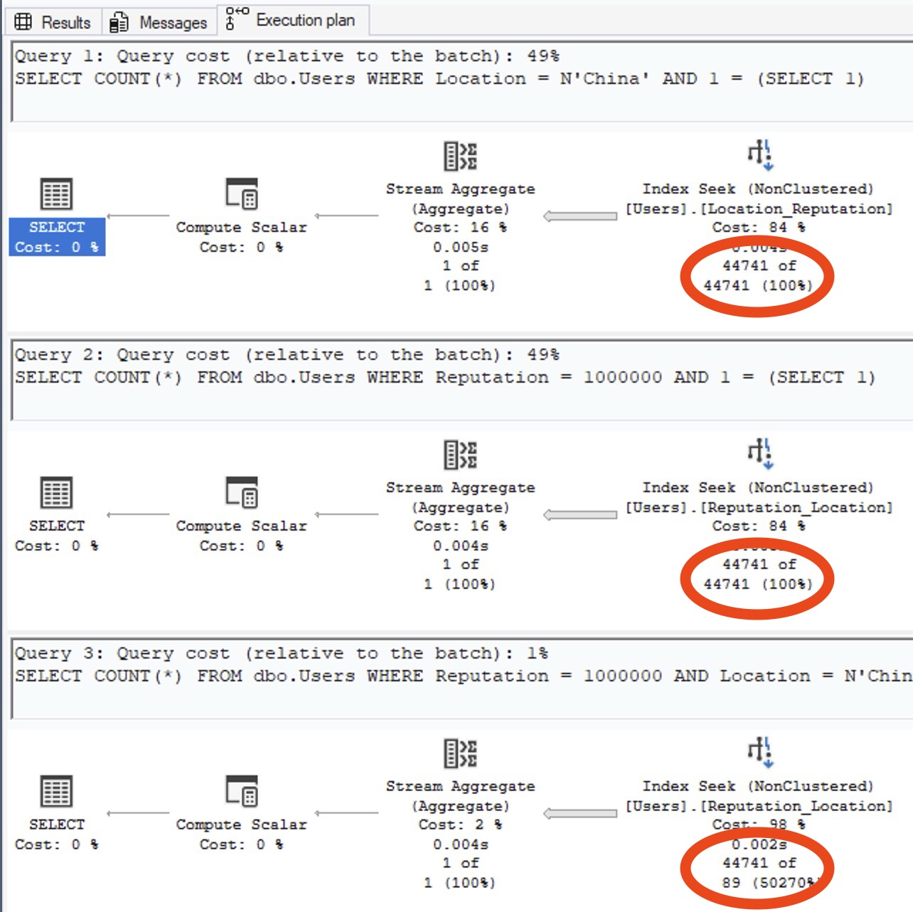
Check out the estimated number of rows on the query plans:
Or for those of you who prefer memes:
If SQL Server had anything even remotely resembling true multi-column stats, the estimate would be closer than this. We don’t, so it’s not.
The documentation suggests that you should create these statistics manually when you know there’s correlation:
|
1 2 3 4 5 6 7 8 9 10 11 12 13 14 15 16 17 18 19 |
CREATE STATISTICS Stat_Location_Reputation ON dbo.Users(Location, Reputation) WITH FULLSCAN; CREATE STATISTICS Stat_Reputation_Location ON dbo.Users(Reputation, Location) WITH FULLSCAN; DBCC FREEPROCCACHE; GO SELECT COUNT(*) FROM dbo.Users WHERE Location = N'China' AND 1 = (SELECT 1); SELECT COUNT(*) FROM dbo.Users WHERE Reputation = 1000000 AND 1 = (SELECT 1); SELECT COUNT(*) FROM dbo.Users WHERE Reputation = 1000000 AND Location = N'China' AND 1 = (SELECT 1); |
But yeah no, that still doesn’t work, and still produces the same 89-row estimate.
To learn how to solve these kinds of problems, check out my Mastering Query Tuning class.

4 Comments. Leave new
Forgive me, I may need more caffeine, but I’m confused by one of your examples. Your first 2 example queries use a variable in the WHERE clause so the values are “unknown” and SQL Server uses the density vectors to estimate 73 rows & 23 rows. Then you use a hard-coded Location and show how SQL Server uses the histogram to estimate 7 rows.
But then you hard-code both Location and Reputation, and SQL Server estimates 7 rows again. But you say, “Exactly the same as if we had a completely unknown location and reputation! SQL Server used the density vector numbers, not the statistics histogram…” If it had used the density vectors, wouldn’t the estimate be 23 rows, same as when you use variables for Location and Reputation?
It’s totally confusing, I get it! This is such a tricky issue. I’ve gone back and tried to clarify the wording to make it more intuitive. Hope that helps!
[…] How Multi-Column Statistics Work (Brent Ozar) […]
Thanks for this. I don’t work with SQL Server anymore, but when I did, there were a few occasions when I tried to fix bad estimates for correlated predicates with multi column stats and, as you’ve shown, it didn’t help. I’m a bit baffled as to what the point of this feature is.